One issue with range and the interquartile range (IQR) both is that they don’t include information from all the data points; the range only considers the two endpoints, and the IQR only considers the third and first quartiles.
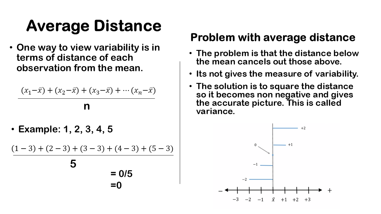
We want a measure of variation that incorporates all the information from data set. One way to achieve this is by considering the average distance of each observation from the mean. This method gives us a sense of how much our data points deviate from the mean on average.
To do this, we take each observation, subtract the mean to find the distance from the mean, sum all these distances or deviations, and then divide by the total sample size. This method provides a comprehensive measure of variability because it considers every data point, giving us a more complete picture of the data’s spread.
For example, consider a set of observations: 1, 2, 3, 4, and 5. The sample size is 5. The mean x̅ is calculated by summing all the values and dividing by the sample size, which gives us 15÷5=3 So, the mean is 3. To measure variation in terms of distances from the mean, we subtract the mean from each observation and then calculate the average of those distances. We have the five observations 1,2,3,4, and 5 and after subtracting the mean 3 we will get -2, -1, 0, 1, 2.

Instead of having five different distances from the mean, we might want an average distance from the mean to make more sense. This would provide a single number representing how far off an observation is from the mean. One way to do this is to take the average of these distances. However, there’s a problem: when you calculate the average of these distances, you end up with a value of zero.
A value of zero is meaningless as a measure of variation or spread in a data set. Clearly, there is some variation, as some points are higher, some are lower, and one point is exactly at the sample mean. Thus, it doesn’t make sense to claim there’s no variation. This simple average of the distances from the mean fails to reflect the variation in the data set.
The issue is that if you take the average of the distances from the mean, it will always equal zero. This approach is flawed because the negative distances below the mean cancel out the positive distances above the mean, and the value at the mean is zero. Essentially, these distances cancel each other out, resulting in an average of zero.
Square the Distance
We aim to measure variability in a way that treats negative distances from the mean as positive or at least non-negative. One effective approach is to square these distances. When you square a number, even if it’s negative, it becomes positive. For instance, squaring -1 results in 1 (since -1 × -1 = 1).
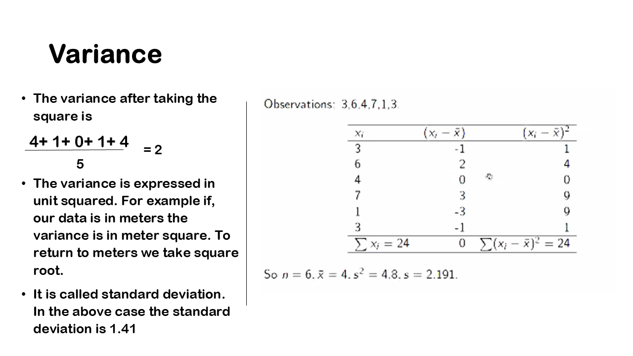
By squaring these deviations from the mean, we transform negative deviations into positive ones. This method ensures that when we sum up these squared values and calculate their average, we obtain a meaningful measure of variability that isn’t confined to zero. This measure is known as variance. It involves squaring each deviation from the mean, summing them, and then averaging them out to provide insight into the spread of data.
In our example, the first deviation is -2, meaning the observation lies two units below the sample mean in negative territory. When we square this value, -2 squared equals 4, which conceptually creates a square or a box with an area of 4. Instead of representing the deviation as -2, we now consider it as a positive square distance of 4 from the mean.
Moving to the next deviation which is one unit below the mean, squaring -1 gives us an area of 1. The observation at the mean itself, 3, has a squared distance of 0 since 0 squared is still 0. The deviation obtained with observation, 4, is one unit above the mean, so squaring 1 result in an area of 1. Finally, for the observation of 5, which is two units above the mean, squaring 2 gives us an area of 4.
Thus, after squaring these deviations, we get values of 4, 1, 0, 1, and 4. By squaring these deviations, we transform negative distances into positive values and maintain positive values as they are. This method allows us to calculate an average of these squared distances, which provides a meaningful measure of variability in the data set.
We can consider the overall variability in this dataset as the sum of these areas of the squares. Adding up the areas of the squares—4 plus 1 plus 0 plus 1 plus 4—gives you a total of 10. This sum represents a snapshot measure of the amount of variation present in this dataset.
Variance of other data

When we average the sum of the squared distances from the mean, we obtain a value of 2. This calculation involves adding up the areas represented by these squared deviations and then dividing by the total number of observations, which is 5. In this context, 10 represents the total variability in our dataset, and 5 is the number of observations. Therefore, as a measure of overall variation, we derive a variance value of 2. Variance is expressed in squared units because we square the distances from the mean during the calculation process.


