Demo Example
Demo Example
Demo Example
Tag

variance

Browsing

Variance represents the average of the squared deviations from the mean. Because we square the deviations, the variance is always a non-negative value, meaning it’s either positive or zero. The method for calculating variance slightly varies depending on whether we are dealing with a sample or a population.

Lets consider an hypothetical example of income, when we analyze income data, we discover that the sample variance is a large figure. Since this is a sample from a population, the sample variance is measured in thousands of rupees squared. This unit, rupees squared, can be challenging to interpret directly. Hence, we prefer using the standard deviation because it will be expressed in rupees, which provides a more intuitive understanding of the variability in the income data.

Key Takeaway 

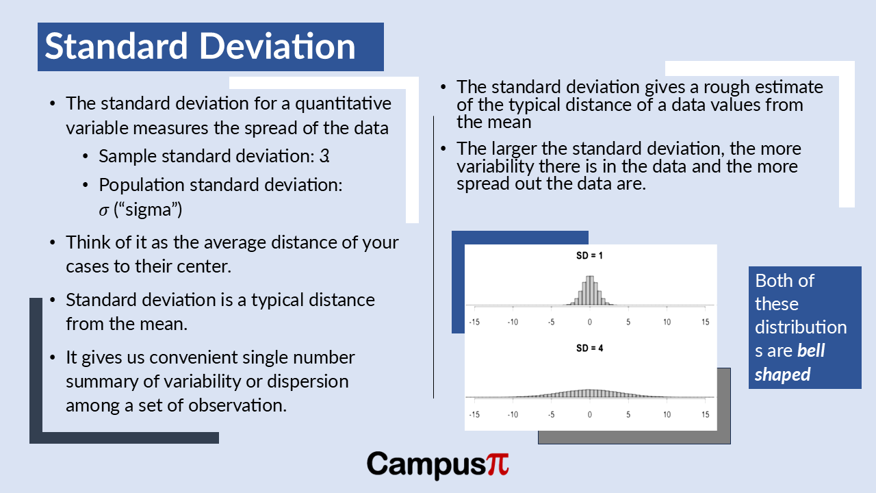
  • The standard deviation represents the typical distance of observations from the mean.
  • When the standard deviation is low, it suggests that most values cluster closely around the mean, indicating less variability.
  • Conversely, a larger standard deviation implies greater variability, with values more spread out from the mean.

Standard Deviation: Population and Sample

When we discuss standard deviation, whether from a population or a sample, the formulas are essentially the same. We simply take the square root of the variance. In the case of population standard deviation, it’s the square root of population variance, and for sample standard deviation, it’s the square root of sample variances.

For our income data, calculating the sample standard deviation is straightforward using statistical software. Taking the square root of our sample variance gives us a standard deviation of approximately 55,000 rupees. This measurement is in the original units of rupees, unlike the sample variance, which is in rupees squared.

Conceptually, the standard deviation provides an indication of the typical distance of our income observations from the sample mean. On average, we can interpret this standard deviation to mean that incomes vary by about 55,000 rupees.

Standard Deviation Interpretation w.r.t Mean
Standard deviation interpretation with respect to mean

To better understand the standard deviation, especially in relation to income or any dataset, it’s helpful to consider its interpretation alongside the mean. The standard deviation represents the typical distance of observations from the mean.

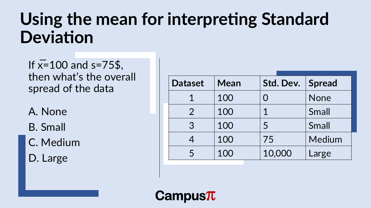
For instance, if we have a dataset with a mean income of INR 100 and a sample standard deviation of INR 0, what does this tell us about the spread of the data? Well, with a standard deviation of zero, it means all values in the dataset are exactly 100. Therefore, the spread of the data in this case would be considered none.

This example illustrates how the mean can aid in interpreting the standard deviation. When the standard deviation is low, it suggests that most values cluster closely around the mean, indicating less variability. Conversely, a larger standard deviation implies greater variability, with values more spread out from the mean. This comparison helps provide a more intuitive understanding of what the standard deviation measures in a dataset.

If we have a sample standard deviation of one rupee and a sample mean of 100, it indicates that the data points are relatively close to the mean. The standard deviation being much smaller than the mean suggests that most observations cluster tightly around the mean value of 100. Therefore, the amount of variability or spread in the data is minimal in this case. A sample mean of 100 and a standard deviation of 5 and is still pretty small there’s not going to be very much variation around the data set.

Suppose our sample mean is 100 and the sample standard deviation is 75. In this case you can say the sample standard deviation is pretty close to the sample mean. So, let’s say that there’s just a medium amount of variability, you can think of it as there are quite a few observations around this sample mean but there is some degree of spread. Finally consider a mean of 100 and a standard deviation of ten thousand then the overall spread of the data it’s going to be large.

We can interpret the sample standard deviation by comparing it with the sample mean. In each scenario we’ve discussed, we’ve kept the sample mean consistent while varying the sample standard deviation.

When the sample standard deviation is significantly large compared to the sample mean, it indicates that the data points are widely spread around the mean. Conversely, if the sample standard deviation is relatively small compared to the sample mean, it suggests there is little variation, meaning most observations are closely clustered around the sample mean. Thus, comparing the standard deviation to the mean helps us gauge the degree of variability in the dataset.

Standard Deviation of Income

Let’s examine our income data to understand what the standard deviation is telling us. The sample standard deviation is 55,000, while the mean income is around 37,000. Since, the sample mean is smaller than the standard deviation, this indicates a relatively large spread around the mean. In other words, these values suggest a significant degree of variability in incomes based on this sample data.

A straightforward solution to deal with unit of variance which is in squared units is to simply calculate the square root of the variance. Since variance is derived from squaring the deviations or distances from the mean, taking its square root reverses this process. Therefore, the square root of the variance gives us a measure of variation known as the standard deviation.

Standard Deviation

Key Takeaway 

  • Standard Deviation can be seen as the average distance from the mean for a set of observations, providing a measure of how spread out the data points are.
  • The square root of the variance gives us a measure of variation known as the standard deviation.
  • The significant advantage of the standard deviation is that it returns us the units in interpretable way for example rather than miles squares in case of variance, just miles.
  • If we examine a dataset with less variability, both the variance and the standard deviation will be smaller.
  • It helps convey the degree of variability in a dataset: the higher the standard deviation, the greater the variability of the observations around the mean.

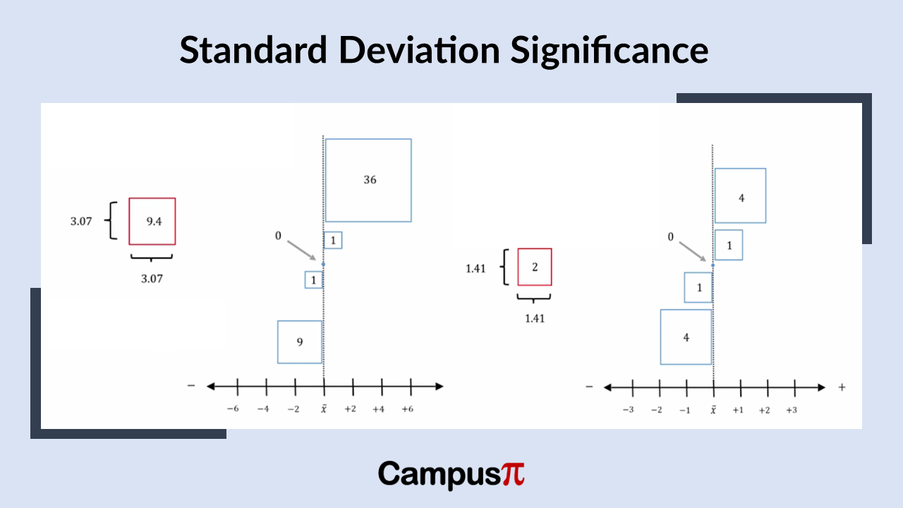
Let’s examine our dataset of one, two, three, four, and five, and consider the significance of the standard deviation. As mentioned earlier, the variance represents the typical size of the boxes that symbolize the squared deviations from the mean. To find the standard deviation, we simply take the square root of the variance. For a dataset where the variance is two, the standard deviation would be approximately 1.41.

The significant advantage of the standard deviation is that it returns us to our original units of measurement. For instance, if our dataset is in miles, the variance would be in square miles, whereas the standard deviation would be in miles, which is more intuitive for interpretation.

What does the standard deviation signify?

Standard Deviation

While the variance indicates the typical squared deviation from the mean, the standard deviation represents the side length of a typical box in our dataset. In this example, with a variance of two, the standard deviation of 1.41 can be seen as the length of one of these boxes. Squaring the standard deviation gives us the variance, demonstrating their mathematical equivalence. However, the preference for the standard deviation lies in its direct association with the original units of measurement, unlike the variance which is in squared units.

If we examine a dataset with less variability, both the variance and the standard deviation will be smaller. For example, in this dataset where the variance is 0.8, the square root of that variance, which is the standard deviation, is 0.9. In other words, the side length of our typical box in this dataset is 0.9. Therefore, the standard deviation of 0.9 reflects the smaller degree of variability present in these observations.

If we examine a dataset with greater variability, the variance will be larger. For instance, if the variance is 9.4, the typical square deviation from the mean is larger, roughly 3. Taking the square root of the variance gives us the standard deviation, which is approximately three.

Degree of variability

The standard deviation is simply the square root of the variance. A larger standard deviation, like one exceeding three, indicates a greater degree of variability in our dataset compared to a standard deviation below one. Thus, the total variability, represented by the variance and standard deviation, changes according to how spread out the data points are from the mean.

Let’s go back to dataset consisting of the values one, two, three, four, and five. These values have distances both above and below the mean. These distances are in their original form and haven’t been squared.

The standard deviation represents the side length of our typical box, which is the typical squared deviation from the mean. When we calculate the standard deviation for this dataset, we get a value of 1.41 units. This length reflects the measure of variability in our dataset.

The standard deviation, when compared to the actual distances or deviations in our dataset, appears quite typical—it’s neither the smallest nor the largest distance from the mean. It can be seen as the average distance from the mean for a set of observations, providing a measure of how spread out the data points are.

In statistical terms, the standard deviation is a clear indicator—it represents a typical deviation or distance from the mean. It helps convey the degree of variability in a dataset: the higher the standard deviation, the greater the variability of the observations around the mean. Unlike simpler measures like the range or interquartile range, both the standard deviation and variance take into account all observations in the dataset.

One of the strengths of the standard deviation is its ability to condense all this information about the observations into a single number, providing a concise summary of the variability or dispersion in the dataset.

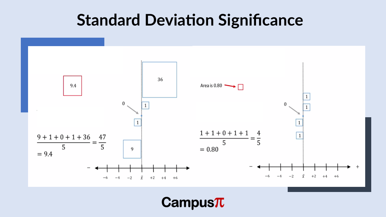
One of the way to measure the variability is to calculate the difference of each observation from the mean. We then square the each distances, sum it and divide by the sample size which gives the variance. Since we square each observation it is represented by the square boxes (which you may have learnt from elementary school) as we can see in the figure. Just to give a reference of amount of variability we can take few examples of deviations with different variances.

Key Takeaway 

  • For a dataset with less variability, the data points are not very different from each other, resulting in a smaller total area occupied by these squares. This means that the sum of the squared deviations or distances from the mean will be smaller.
  • Dataset with greater variability, occupies more space when we sum up the areas of the squares. In simpler terms, for a dataset with more variability, the sum of the squared distances from the mean is higher.
  • The units of variance are in squared units, meaning if the original dataset uses miles as units, the variance would be in square miles; if it’s in inches, the variance would be in square inches. This reflects how we calculate variance by squaring the deviations from the mean.
  • Interpreting variance can be challenging to interpret directly in terms of the original unit of measurement. For instance, if our dataset is in Miles, it’s more intuitive to understand variability in Miles rather than Miles squared.

For a dataset with less variability, the data points are not very different from each other, resulting in a smaller total area occupied by these squares. This means that the sum of the squared deviations or distances from the mean will be smaller. In the above example, the sum of the squared deviations from the mean is 9 plus 1 plus 0 plus 1 plus 36 which is 47 and 1 plus 1 plus 0 plus 1 plus 1, which equals 4. Visually, you can see that the area covered by the squares is smaller for the chart in right side than left side.

Variance

When you examine a dataset with greater variability, it occupies more space when you sum up the areas of the squares. In simpler terms, for a dataset with more variability, the sum of the squared distances from the mean is higher. This sum, which represents the area covered by the squares after squaring the distances from the mean, encapsulates the extent of variation within the dataset. Conversely, a dataset with less variability would have a smaller sum of squared distances.

To quantify this variation with a single measure, we use the variance, which is calculated by dividing the sum of the squared distances from the mean by the sample size. Importantly, variance indicates the variability present in our dataset.

If we examine the dataset with less overall variability, we see that the total area covered by the boxes is smaller. In this case, the typical box representing the variance has an area of 0.8. In simpler terms, when the total variability is reduced, the variance also decreases. For this example, the total variation, calculated as the sum of squared deviations from the mean (1 + 1 + 0 + 1 + 1) divided by five, equals 0.8.

So, that’s how variance is determined for a dataset. A dataset with higher variability results in a slightly larger box, as seen in this case where the variance is 9.4. The typical box representing the variance for this dataset is 9.4 in area. This calculation remains consistent: total variability divided by the number of observations gives us this value of 9.4.

The variance effectively serves as the average of the sum of squared deviations from the mean. It accurately reflects the level of variability within a dataset: a higher variance value indicates greater variability among observations, while a lower variance value indicates less variability.

Unit of Variance

The units of variance are in squared units, meaning if the original dataset uses miles as units, the variance would be in square miles; if it’s in inches, the variance would be in square inches. This reflects how we calculate variance by squaring the deviations from the mean.

However, this drawback of the variance as it’s presented in squared units, can be challenging to interpret directly in terms of the original unit of measurement. For instance, if our dataset is in Miles, it’s more intuitive to understand variability in Miles rather than Miles squared.

This highlights a key issue with variance: its unit of measure squared makes interpretation less straightforward. Instead, a more practical approach would be to use a measure of variability that directly reflects the original unit of measurement. For example, instead of inches squared, we would prefer a measure based on inches; similarly, for Miles squared, we would prefer a measure based on Miles. A solution to this is to take square root of variance which is also know as standard deviation.